PyMP Tutorial 0. Manipulating Objects

Manipulating Signals

First thing you may want to do is load, analyse, plot and write signals. These operations are handled using the Signal class.

Reading and Writing

You can use the constructor of the Signal class to load a wav file from the disk. This is internally done using the wave python module shipped with the standard library. Assuming you’ve correctly set the PYTHONPATH variable so that it contains the pymp/PyMP/ directory, you can simply type in a python shell:

>>> from PyMP import Signal
>>> signal = Signal('data/glocs.wav')

As for many pymp Objects, you can specify a debug level that manages info and warning printing degrees. Try for example:

>>> signal =  Signal('data/glocs.wav', debug_level=3)
>>> print signal
Signal object located in data/glocs.wav
        length: 276640
        energy of 271319943.000
        sampling frequency 32000
        number of channels 1

The Signal object signal wraps the content of glocs.wav as a numpy array and descriptors such as sampling frequency, sample format, etc.. you can access the samples directly as a numpy array by doing:

>>> signal.data
array([[  0],
       [  0],
       [  0],
       ...,
       [-38],
       [-41],
       [-44]], dtype=int16)

Meaning you can also create a Signal object directly from a numpy array:

>>> import numpy as np
>>> zero_signal = Signal(np.zeros((1024,)), Fs=8000)

where Fs is the sampling frequency (default is zero)

Visualizations

At any moment you can visualize the data using the Signal.plot() function:

>>> signal.plot()

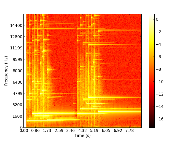
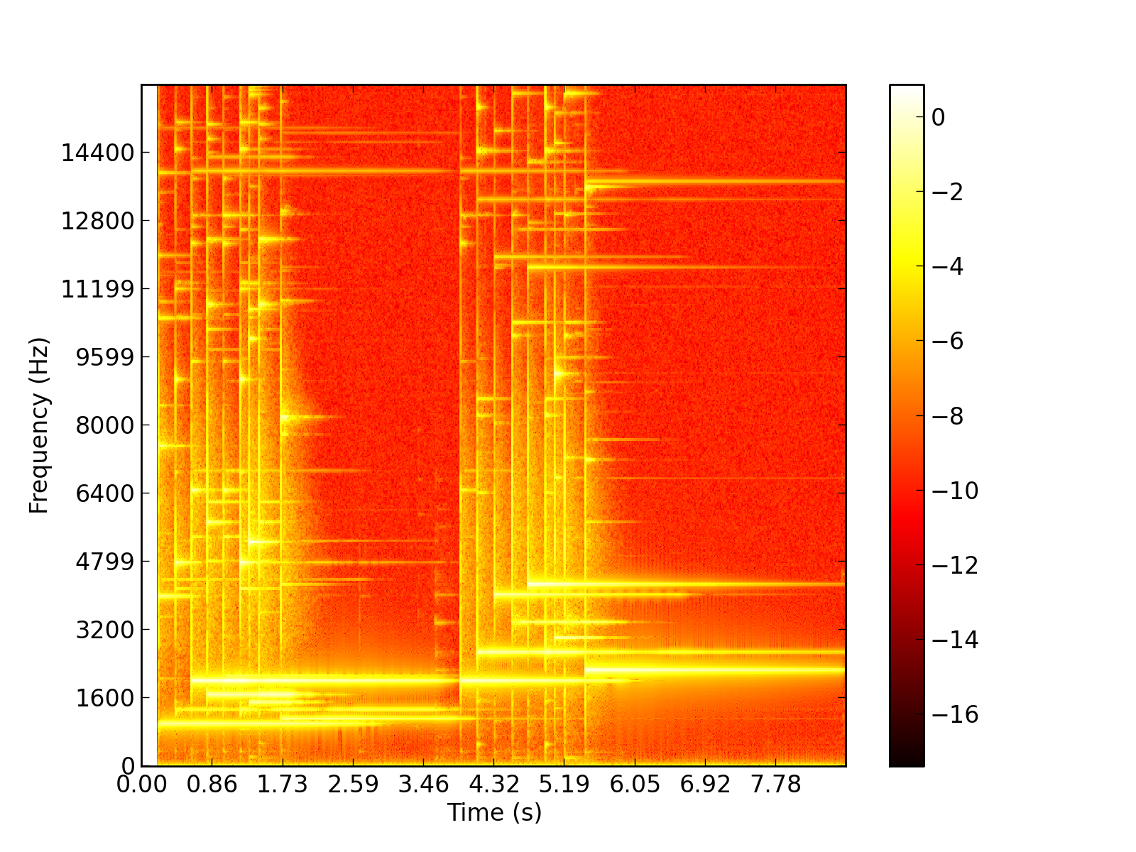
Alternatively, a useful routine to visualize the time-frequency content is the Signal.spectrogram() function. For instance, to plot the logarithm of the power spectrum with a 1024 sample window and 75% overlap:

>>> signal.spectrogram(1024, 256, order=2, log=True, cmap=cm.hot, cbar=True)

(Source code, png, hires.png, pdf)

Writing a signal is also quite straightforward:

>>> signal.write('new_dest_file.wav')

Signal Edition

Often you need to edit signals, e.g. crop them or pad them with zeroes on the borders, this can be done easily:

>>> print signal.length
276640

>>> signal.crop(0 , 2048)
>>> print signal.length
2048

Another way is to use:

>>> sub_signal = signal[0: 2048]
>>> print sub_signal
Signal object located in
        length: 2048
        energy of 0.000
        sampling frequency 32000
        number of channels 1

Revesely you can pad signals with zeroes, this is done on both sides with pad and depad methods. For example, we can create a signal with only ones and pad it with zeroes on the edges:

>>> signal = Signal(np.ones((8,)), 1)
>>> signal.data
array([ 1.,  1.,  1.,  1.,  1.,  1.,  1.,  1.])

>>> signal.pad(4)
>>> signal.data
array([ 0.,  0.,  0.,  0.,  1.,  1.,  1.,  1.,  1.,  1.,  1.,  1.,  0.,
        0.,  0.,  0.])

Removing the zeroes is also straightforward:

>>> signal.depad(4)
>>> signal.data
array([ 1.,  1.,  1.,  1.,  1.,  1.,  1.,  1.])

Manipulating Approximation objects

Note

Approx objects are the equivalent of Book objects in MPTK. They handle the approximation of a signal on a given dictionary.

Creation

A trivial creation takes no further arguments.

>>> from PyMP.approx import Approx
>>> approx = Approx()

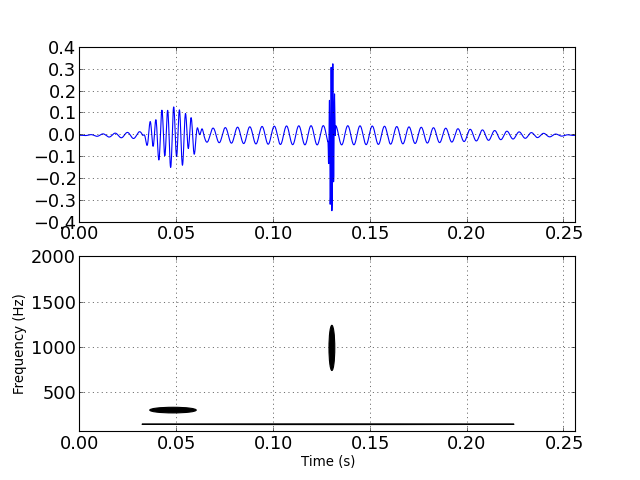
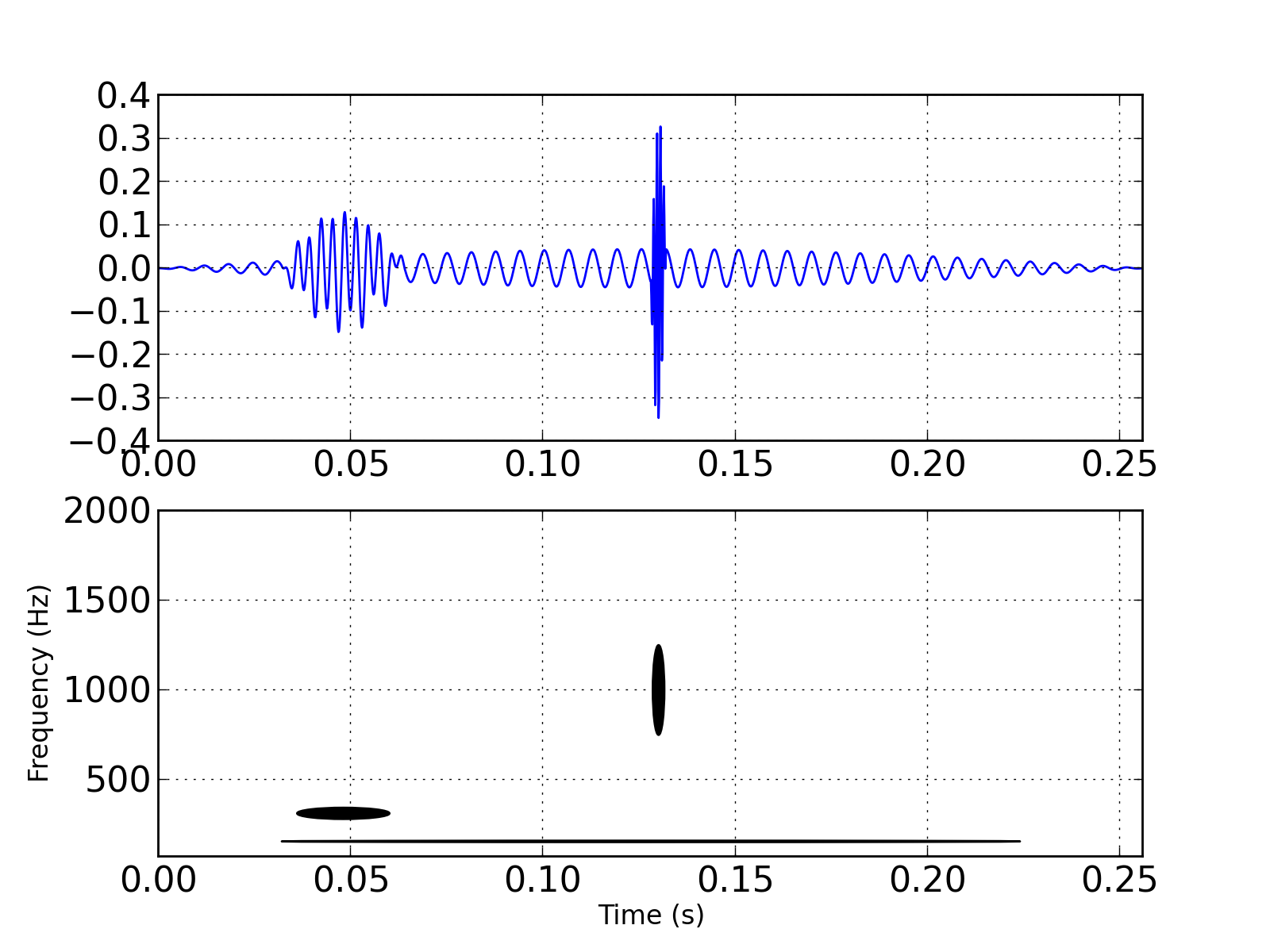
Basically, an approximant is just a collection of atoms, this means we can enrich this object py adding some atoms to it. For example we can add 3 MDCT atoms of different scales, time and frequency localization to obtain an approximant as in the following example:

(Source code, png, hires.png, pdf)

This example use the Atom objects. The long atom (2048 samples or 256 ms at a sampling rate of 8000 Hz) is built using the command:

>>> from PyMP.mdct.atom import Atom
>>> atom_long = Atom(2048, 1, 0, 40, 8000, 1)

where we have specified its size, amplitude (Deprecated, always put 1 in there) , time localization (0) , frequency bin (40 which corresponds to 156 Hz) and mdct_coefficient value (1) then the atom’s waveform is synthesized using internal routine and used to create a Approx object:

>>> atom_long.synthesize()
>>> approx  = Approx(None, [], None, atom_long.length, atom_long.fs)
>>> print approx
Approx Object: 0 atoms, SRR of 0.00 dB

Other atoms can be added:

>>> approx.add(Atom(256, 1, 256, 10, 8000, 1))
>>> print approx
Approx Object: 1 atoms, SRR of 0.00 dB

Approximation in a MP context

Although you can manipulate Approx objects on their own, it is much more interesting to link them to existing signals and to a dictionary. For example, let us define a dictionary as a union of 3 MDCT basis:

>>> from PyMP import Signal
>>> from PyMP.mdct import Dico
>>> dico = Dico([128,1024,8192])

We can now create an approximation of a specified signal on this dictionary this way:

>>> signal = Signal('data/glocs.wav',mono=True)
>>> approx = Approx(dico, [], signal)

for now this approximation is empty (the approx.atoms list is empty). But we can still add an atom to it:

>>> approx.add(Atom(256, 1, 256, 10, 8000, 1))
>>> print approx
Approx Object: 1 atoms, SRR of 0.00 dB

Now we have a reference signal and an approximant of it, we can evaluate the quality of the approximation using the Signal to Residual Ratio (SRR):

>>> print approx.compute_srr()
-116.636999534

Since we picked a random atom with no link to the signal, the SRR (in dB) is very poor. It will be much better when MP select atoms based on their correlation to the signal