PyMP Tutorial 1. MP decomposition with Unions of MDCT

This tutorial will describe how PyMP works, and mostly how to use it to perform audio signal decompositions on multiscale MDCT dictionaries for any question feel free to contact me (firstname.lastname@gmail.com) Documentation for the modules that we’re using here is provided in the next sections.

Standard Algorithm

In this example, the standard algorithm is used to decomposed the glockenspiel signal over a union of 3 MDCT basis:

>>> import numpy as np
>>> from PyMP import Signal, mp
>>> from PyMP.approx import Approx
>>> from PyMP.mdct import Dico
>>> scales = [128, 1024, 8192]
>>> n_atoms = 500
>>> srr = 50
>>> signal = Signal('data/glocs.wav', mono=True, normalize=True)
>>> signal.crop(0, 3.5 * signal.fs)
>>> signal.pad(8192)
>>> dico = Dico(scales)
>>> approx, decay = mp.mp(signal, dico, srr, n_atoms)

Note

IMPORTANT: the fact that we know it’s the standard algorithm that is used is because we choosed a Dico object as dictionary.

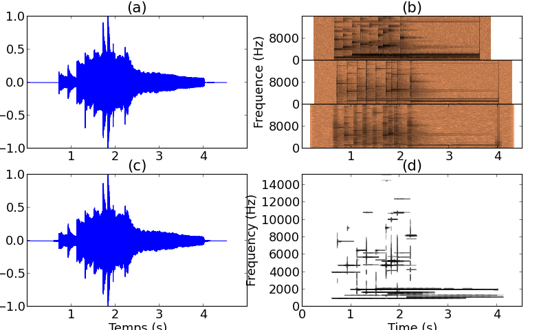
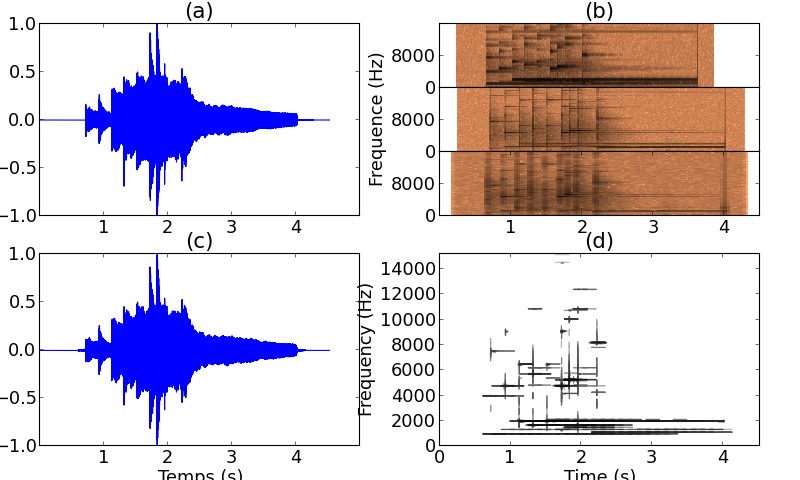
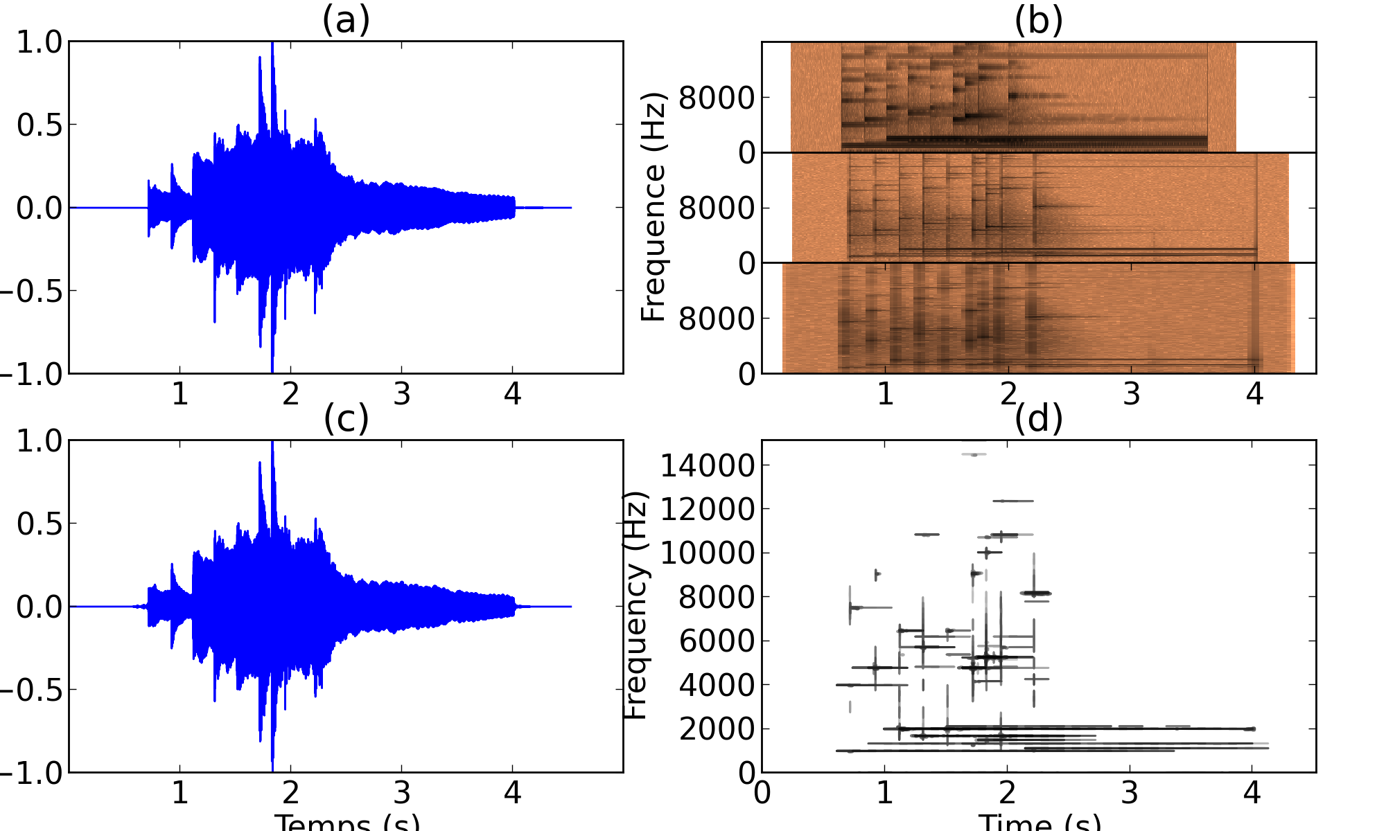
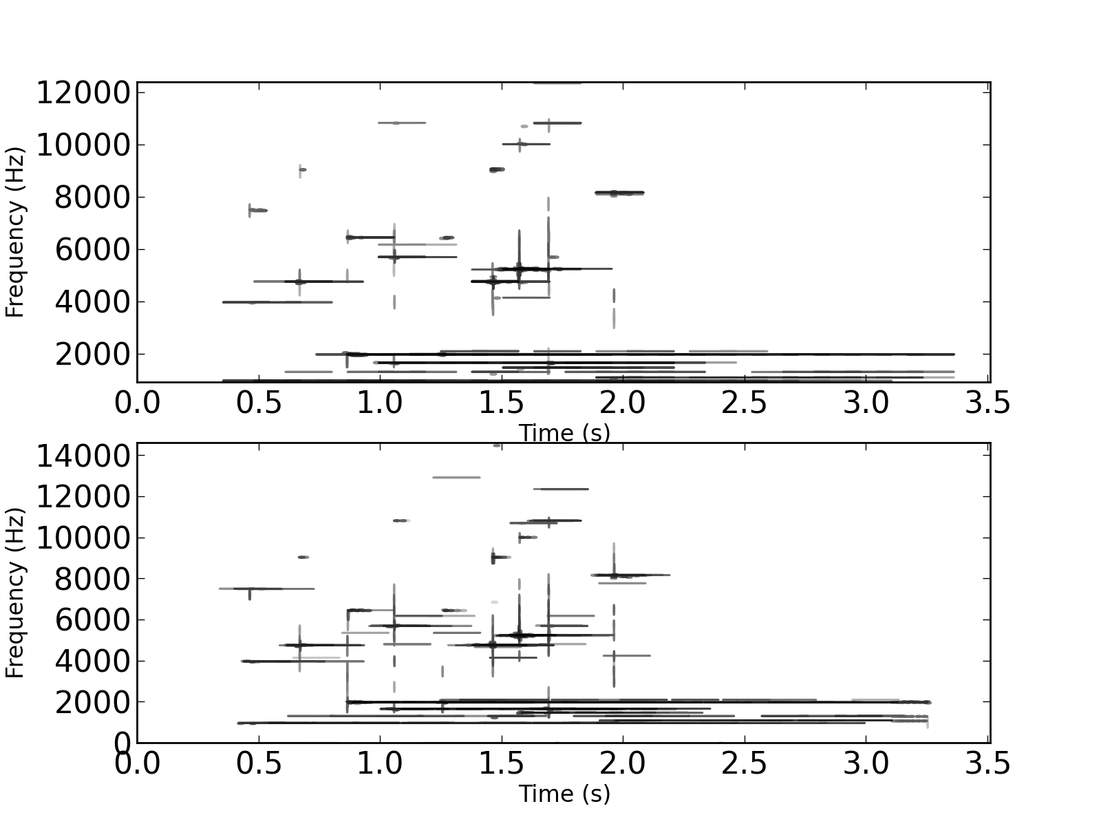
First plot (a) is the original glockenspiel waveform. (b) presents the 3 MDCT (absolute values) considered. (c) is the reconstructed signal, accessible via:

>>> approx.recomposed_signal
Signal object located in
        length: 144768
        energy of 1812.389
        sampling frequency 32000
        number of channels 1

and (d) is the time-frequency plot of the 1000 atoms that have been used to approximate the original glockenspiel signal

(Source code, png, hires.png, pdf)

You can evaluate the quality of the approximation:

>>> approx.compute_srr() 
19.167848...

and save the result in various formats (see the Approx documentation):

>>> approx.recomposed_signal.write('outPutPath.wav')

Locally Optimized MP

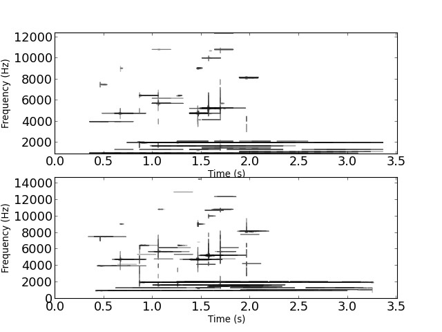
To run a locally adaptive (or optimized) MP, all we have to do is to pick a LODico object as a dictionary. The internal routines of its blocks will perform the local optimization so that at our level this is quite transparent:

>>> from PyMP.mdct import LODico
>>> mp_approx, mp_decay = mp.mp(signal, Dico(scales), srr, n_atoms, pad=True)
>>> lomp_approx, lomp_decay = mp.mp(signal, LODico(scales), srr, n_atoms, pad=True)

(Source code, png, hires.png, pdf)

In addition to plotting, we can compare the quality of the approximations, given a fixed number of atoms (here 500):

>>> print mp_approx
Approx Object: 500 atoms, SRR of 19.17 dB
>>> print lomp_approx
Approx Object: 500 atoms, SRR of 23.27 dB

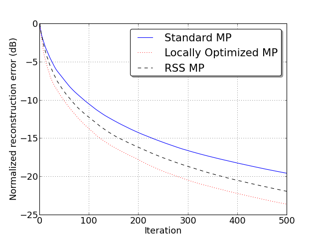
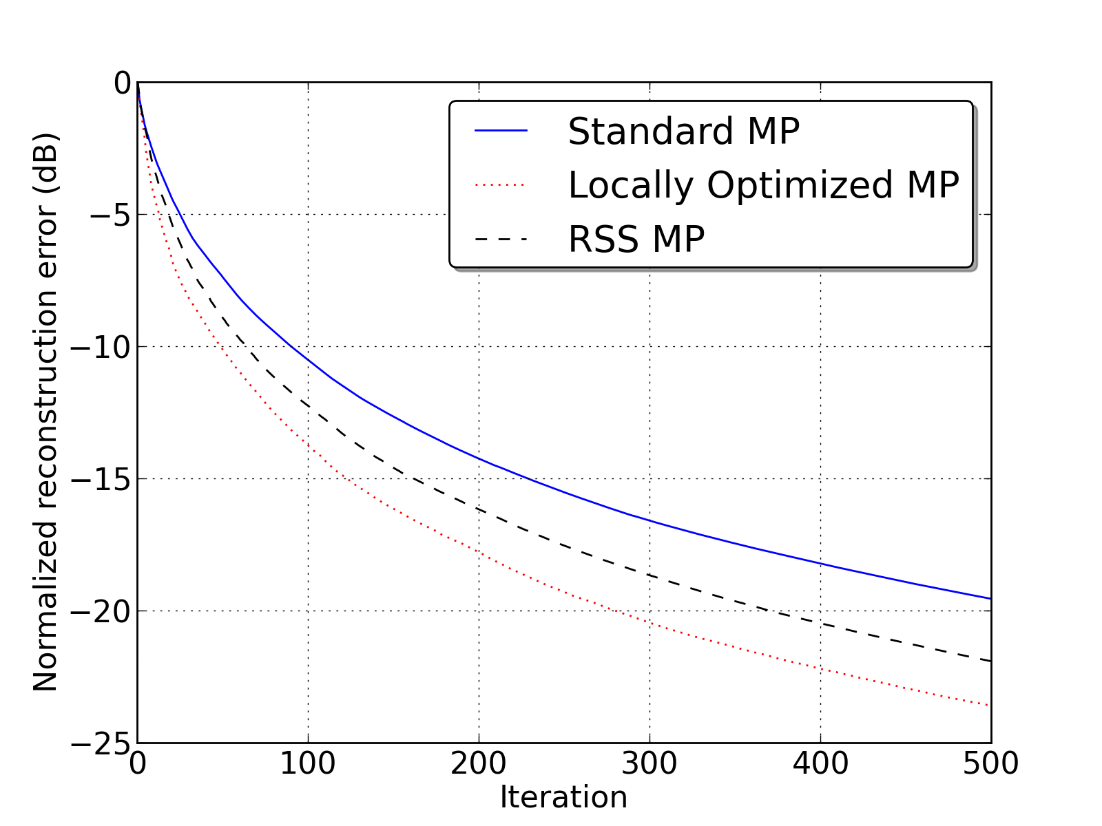
The locally adaptive Matching pursuit has yielded a better decomposition (in the sense of mean squared error). Alternatively one can verify that for a given level of SRR, LoMP will use a smaller number of atoms.

MP with Random Sequential Subdictionaries

RSSMP is explained in the journal paper .

Implementation of RSSMP is quite transparent, it’s done through the use of a SequenceDico object as dictionary:

>>> from PyMP.mdct.rand import SequenceDico
>>> seq_dico = SequenceDico(scales, 'random')

We can now compare the three strategies in terms of normalized reconstruction error

This gives the following results:

(Source code, png, hires.png, pdf)

And that’s it.